Finite difference Poisson equation
Full Poisson problem: Dirichlet boundary conditions
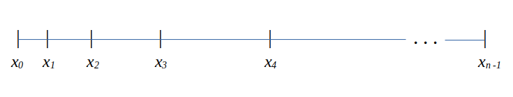
Let’s consider the boundary conditions and grading ratio are,
(16)\[\begin{split}\begin{aligned}
\phi{(x_0)} = left\ bc = 0;\\
\phi{(x_{n-1})} = right\ bc = 0;\\
\Delta{x_i} = x_{i+1} - x_i = r\Delta{x_{i-1}};\\
r = Grading\ ratio =\frac{\Delta{x_i}}{\Delta{x_{i-1}}};
\end{aligned}\end{split}\]
Now, using Taylor series expansion at \(\phi_{i+1}\) we get,
(17)\[\phi_{i+1} = \phi_i+(\Delta x_i) \frac{\partial \phi}{\partial x}|_{i}+\frac{\Delta x_i^2}{2!}\frac{\partial^2\phi}{\partial x^2}|_i + \frac{\Delta x_i^3}{3!}\frac{\partial^3\phi}{\partial x^3}|_i + ......\]
And, using Taylor series expansion at \(\phi_{i-1}\) we get,
(18)\[\phi_{i-1} = \phi_i-(\Delta x_{i-1}) \frac{\partial \phi}{\partial x}|_{i}+\frac{\Delta x_{i-1}^2}{2!}\frac{\partial^2\phi}{\partial x^2}|_i - \frac{\Delta x_{i-1}^3}{3!}\frac{\partial^3\phi}{\partial x^3}|_i + ......\]
Multiplying equation (18) by \(r\) and adding with equation (17) we get,
(19)\[\phi_{i+1}+r\phi_{i-1} = (1+r)\phi_i+(\Delta x_i - r\Delta x_{i-1})\frac{\partial \phi}{\partial x}|_{i} +\frac{(\Delta x_i)^2 + r(\Delta x_{i-1})^2}{2}\frac{\partial^2\phi}{\partial x^2}|_i\]
Since \(\Delta{x_i} = r\Delta{x_{i-1}}\), second term of the right hand side is eliminated and we get,
(20)\[\phi_{i+1}+r\phi_{i-1} = (1+r)\phi_i+\frac{(\Delta x_i)^2 + r(\Delta x_{i-1})^2}{2}\frac{\partial^2\phi}{\partial x^2}|_i\]
(21)\[=> r\phi_{i-1}-(r+1)\phi_i+\phi_{i+1} = \frac{(\Delta x_i)^2 + r(\frac{\Delta x_{i}}{r})^2}{2}\frac{\partial^2\phi}{\partial x^2}|_i\]
(22)\[=> r\phi_{i-1}-(r+1)\phi_i+\phi_{i+1} = \frac{(\Delta x_i)^2 + \frac{(\Delta x_{i})^2}{r}}{2}\frac{\partial^2\phi}{\partial x^2}|_i\]
(23)\[=> \frac{\partial^2\phi}{\partial x^2}|_i = \frac{r\phi_{i-1}-(r+1)\phi_i+\phi_{i+1}}{(\frac{r+1}{2r})(\Delta x_i)^2}\]
(24)\[=> \frac{\partial^2\phi}{\partial x^2}|_i = \frac{(\frac{2r^2}{r+1})\phi_{i-1}-2r\phi_i+(\frac{2r}{r+1})\phi_{i+1}}{(\Delta x_i)^2}\]
So, the discrete finite difference form of equation (15) is,
(25)\[=> \frac{\partial^2\phi}{\partial x^2}|_i = \frac{(\frac{2r^2}{r+1})\phi_{i-1}-2r\phi_i+(\frac{2r}{r+1})\phi_{i+1}}{(\Delta x_i)^2} = -(\frac{\rho}{\epsilon_0})_i\]
Corresponding stencil is \(((\frac{2r^2}{r+1}), -2r, (\frac{2r}{r+1}))\).
So, the system of linear equations are,
\[\label{eq_2nddev12}
\phi_0 = 0;\]
\[\label{eq_2nddev13}
(\frac{2r^2}{r+1})\phi_0-2r\phi_1+(\frac{2r}{r+1})\phi_2 = (\Delta x_1)^2 (-(\frac{\rho}{\epsilon_0})|_1);\]
\[\label{eq_2nddev14}
(\frac{2r^2}{r+1})\phi_1-2r\phi_2+(\frac{2r}{r+1})\phi_3 = (\Delta x_2)^2 (-(\frac{\rho}{\epsilon_0})|_2);\]
\[\label{eq_2nddev15}
(\frac{2r^2}{r+1})\phi_2-2r\phi_3+(\frac{2r}{r+1})\phi_4 = (\Delta x_3)^2 (-(\frac{\rho}{\epsilon_0})|_3);\]
\[\begin{split} \label{eq_2nddev16}
.......................................\\
.......................................\end{split}\]
\[\label{eq_2nddev17}
(\frac{2r^2}{r+1})\phi_{n-3}-2r\phi_{n-2}+(\frac{2r}{r+1})\phi_{n-1} = (\Delta x_{n-2})^2 (-(\frac{\rho}{\epsilon_0})|_{n-2});\]
\[\label{eq_2nddev18}
\phi_{n-1} = 0;\]
Corresponding matrix-vector representation of system of linear equations will be,
(26)\[Ax = b\]
Where, the matrix \(A\) is,
(27)\[\begin{split}A = \begin{vmatrix}
1&0&0&0&..&..&..&0\\
\frac{2r^2}{(r+1)}&-2r&\frac{2r}{r+1}&0&0&..&..&..\\
0&\frac{2r^2}{(r+1)}&-2r&\frac{2r}{r+1}&0&..&..&..\\
..&..&..&..&..&..&..&..\\
..&..&..&..&..&..&..&..\\
0&..&..&..&..&\frac{2r^2}{(r+1)}&-2r&\frac{2r}{r+1}\\
0&0&..&..&..&..&0&1\\
\end{vmatrix}\end{split}\]
The vector \(\vec x\) is,
(28)\[\begin{split}\vec x = \begin{vmatrix}
\phi_0\\
\phi_1\\
\phi_2\\
..\\
..\\
\phi_{n-2}\\
\phi_{n-1}
\end{vmatrix}\end{split}\]
The vector \(\vec b\) is,
(29)\[\begin{split}\vec b = \begin{vmatrix}
0\\
-((\Delta x_1)^2 (\frac{\rho}{\epsilon_0})_1)\\
-((\Delta x_2)^2 (\frac{\rho}{\epsilon_0})_2)\\
..\\
..\\
-((\Delta x_{n-2})^2 (\frac{\rho}{\epsilon_0})_{n-2})\\
0
\end{vmatrix} + \begin{vmatrix}
left \ bc\\
0\\
0\\
..\\
..\\
0\\
right \ bc
\end{vmatrix}\end{split}\]
(30)\[\begin{split}=> \vec b = \begin{vmatrix}
left \ bc\\
-((\Delta x_1)^2 (\frac{\rho}{\epsilon_0})_1)\\
-((\Delta x_2)^2 (\frac{\rho}{\epsilon_0})_2)\\
..\\
..\\
-((\Delta x_{n-2})^2 (\frac{\rho}{\epsilon_0})_{n-2})\\
right \ bc
\end{vmatrix}\end{split}\]
Therefore the \(A \vec x = \vec b\) system of equations will be,
(32)\[\begin{split}\begin{vmatrix}
1&0&0&0&..&..&..&0\\
\frac{2r^2}{(r+1)}&-2r&\frac{2r}{r+1}&0&0&..&..&..\\
0&\frac{2r^2}{(r+1)}&-2r&\frac{2r}{r+1}&0&..&..&..\\
..&..&..&..&..&..&..&..\\
..&..&..&..&..&..&..&..\\
0&..&..&..&..&\frac{2r^2}{(r+1)}&-2r&\frac{2r}{r+1}\\
0&0&..&..&..&..&0&1\\
\end{vmatrix}
\begin{vmatrix}
\phi_0\\
\phi_1\\
\phi_2\\
..\\
..\\
\phi_{n-2}\\
\phi_{n-1}
\end{vmatrix} = \begin{vmatrix}
left \ bc\\
-((\Delta x_1)^2 (\frac{\rho}{\epsilon_0})_1)\\
-((\Delta x_2)^2 (\frac{\rho}{\epsilon_0})_2)\\
..\\
..\\
-((\Delta x_{n-2})^2 (\frac{\rho}{\epsilon_0})_{n-2})\\
right \ bc
\end{vmatrix}\end{split}\]
This is for Dirichlet boundary condition on both ends.
1D Full Poisson problem: Neumann boundary condition
Let’s consider the Neumann boundary condition on left boundary,
\[\frac{\partial \phi}{\partial x} = g\]
Where, \(g\) is the value of the derivative at the boundary.
Now, to deal the boundary simply, we consider a ghost node at the left of \(x_0\) so that, \(x_0 - x_{-1} = x_1 - x_0\), that is,
even though our mesh is nonuniform (graded), we consider uniform grid for ghost node. This will make calculation easier for boundary condition.
So, now using central difference scheme on the boundary node and considering direction as towards left, this equation can be written as,
\[\begin{split}\frac{\phi_{-1} - \phi_1}{2\Delta x_0} = g \notag \\
\implies \phi_{-1} = 2 \Delta x_0 g + \phi_1\end{split}\]
Considering a ghost node at \(x_{-1}\) and uniform mesh for first three nodes, at the boundary node we can write,
\[\begin{split}\frac{\phi_{-1} - 2\phi_0 + \phi_1}{(\Delta x_0)^2} = (-(\frac{\rho}{\epsilon_0})|_0) \notag \\
\implies \phi_{-1} - 2\phi_0 + \phi_1 = \Delta x_0^2 (-(\frac{\rho}{\epsilon_0})|_0) \notag \\
\implies 2\Delta x_0 g + \phi_1 -2\phi_0 + \phi_1 = \Delta x_0^2 (-(\frac{\rho}{\epsilon_0})|_0) \notag \\
\implies -2 \phi_0 + 2\phi_1 = \Delta x_0^2 (-(\frac{\rho}{\epsilon_0})|_0) - 2\Delta x_0\ g\end{split}\]
Similar treatment at right boundary gives,
\[2x_{n-2} - 2x_{n-1} = \Delta x_{n-2}^2 (-(\frac{\rho}{\epsilon_0})|_{n-1}) - 2\Delta x_{n-2}\ g\]
Therefore the \(A\vec x = \vec b\) system of equations will be,
(32)\[\begin{split}\begin{vmatrix}
-2&2&0&0&..&..&..&0\\
\frac{2r^2}{(r+1)}&-2r&\frac{2r}{r+1}&0&0&..&..&..\\
0&\frac{2r^2}{(r+1)}&-2r&\frac{2r}{r+1}&0&..&..&..\\
..&..&..&..&..&..&..&..\\
..&..&..&..&..&..&..&..\\
0&..&..&..&..&\frac{2r^2}{(r+1)}&-2r&\frac{2r}{r+1}\\
0&0&..&..&..&..&2&-2\\
\end{vmatrix}
\begin{vmatrix}
\phi_0\\
\phi_1\\
\phi_2\\
..\\
..\\
\phi_{n-2}\\
\phi_{n-1}
\end{vmatrix} = \begin{vmatrix}
-((\Delta x_0)^2 (\frac{\rho}{\epsilon_0})_0) - 2g\Delta x_0\\
-((\Delta x_1)^2 (\frac{\rho}{\epsilon_0})_1)\\
-((\Delta x_2)^2 (\frac{\rho}{\epsilon_0})_2)\\
..\\
..\\
-((\Delta x_{n-2})^2 (\frac{\rho}{\epsilon_0})_{n-2})\\
-((\Delta x_{n-2})^2 (\frac{\rho}{\epsilon_0})_{n-1}) - 2g\Delta x_{n-2}
\end{vmatrix}\end{split}\]
This is for Neumann boundary condition on both ends.
Please note that, we can’t set both the boundaries as Neumann in the implementation at the moment.
At least one should be Dirichlet for now.
1D Boltzmann electron problem
For Boltzmann electrons, equation (15) will be,
\[\Delta^2 \phi (x) = -\frac{\rho}{\epsilon_0} + \frac{n_0 e}{\epsilon_0}\ exp\ (\frac{e\phi}{k_B T_e})\]
Where \(n_0\) is the electron density, \(e\) is the elementary charge, \(k_B\) is the Boltzmann constant and \(T_e\) is the electron temperature.
Following similar treatment for nonuniform mesh, using equation (25) we can write,
\[\begin{split}\frac{\partial^2\phi}{\partial x^2}|_i = \frac{(\frac{2r^2}{r+1})\phi_{i-1}-2r\phi_i+(\frac{2r}{r+1})\phi_{i+1}}{(\Delta x_i)^2} = -(\frac{\rho}{\epsilon_0})_i + \frac{n_0 e}{\epsilon_0}\ exp\ (\frac{e\phi_i}{k_B T_e}) \notag \\
\implies (\frac{2r^2}{r+1})\phi_{i-1}-2r\phi_i+(\frac{2r}{r+1})\phi_{i+1} = -(\frac{\rho}{\epsilon_0})_i (\Delta x_i)^2 + \frac{n_0 e}{\epsilon_0} (\Delta x_i)^2 \ exp\ (\frac{e\phi_i}{k_B T_e}) \notag \\
\implies (\frac{2r^2}{r+1})\phi_{i-1}-2r\phi_i+(\frac{2r}{r+1})\phi_{i+1} + (\frac{\rho}{\epsilon_0})_i (\Delta x_i)^2 - \frac{n_0 e}{\epsilon_0} (\Delta x_i)^2 \ exp\ (\frac{e\phi_i}{k_B T_e}) = 0 \notag \\
\implies F(\phi_i) = (\frac{2r^2}{r+1})\phi_{i-1}-2r\phi_i+(\frac{2r}{r+1})\phi_{i+1} + (\frac{\rho}{\epsilon_0})_i (\Delta x_i)^2 - \frac{n_0 e}{\epsilon_0} (\Delta x_i)^2 \ exp\ (\frac{e\phi_i}{k_B T_e}) = 0 \notag\end{split}\]
Considering \(\vec \phi = (\phi_0, \phi_1, ....., \phi_{n-1})^t\), we need to solve the following equation for \(\phi_i\),
(33)\[F_i(\vec{\phi}) = (\frac{2r^2}{r+1})\phi_{i-1}-2r\phi_i+(\frac{2r}{r+1})\phi_{i+1} + (\frac{\rho}{\epsilon_0})_i (\Delta x_i)^2 - \frac{n_0 e}{\epsilon_0} (\Delta x_i)^2 \ exp\ (\frac{e\phi_i}{k_B T_e})\]
This is a nonlinear problem and we can solve it using Newton-Raphson method. With some initial guess \(x^0\), accoding to Newton-Raphson method, consecutive iterative solution will be,
\[x^{n+1} = x^{n} - \frac{f(x^{n})}{f^{'}(x^{n})}
\implies f^{'}(x^{n}) (x^{n} - x^{n+1}) = f(x^{n})\]
For system of equations \(f(\vec x) = \vec(0)\), this equation becomes,
\[f^{'}(\vec x^n) (\vec x^n - \vec x^{n+1}) = f(\vec x^n)\]
Considering, \(\delta \vec x = \vec x^n - \vec x^{n+1}\), the equation becomes,
\[\begin{split}f^{'}(\vec x^n) \delta \vec x = f(\vec x^n) \notag \\
\implies \frac{\partial f(\vec x^n)}{\partial \vec x^n} \delta \vec x = f(\vec x^n)\end{split}\]
Applying this treatment on equation (33) for \(i^{th}\) term of potential, we can write,
(34)\[\begin{split}(\frac{2r^2}{r+1})\delta \phi_{i-1}-2r\delta \phi_i+(\frac{2r}{r+1})\delta \phi_{i+1} - \frac{n_0 e^2}{\epsilon_0 k_B T_e} (\Delta x_i)^2 \delta \phi_i \ exp\ (\frac{e\phi^n_i}{k_B T_e}) = \notag \\ (\frac{2r^2}{r+1})\phi^n_{i-1}-2r\phi^n_i+(\frac{2r}{r+1})\phi^n_{i+1} + (\frac{\rho}{\epsilon_0})_i (\Delta x_i)^2 - \frac{n_0 e}{\epsilon_0} (\Delta x_i)^2 \ exp\ (\frac{e\phi^n_i}{k_B T_e})\end{split}\]
Solving this equation for \(\delta \vec \phi\) for all nodes and computing \(\vec \phi^{n+1} = \vec \phi^n - \delta \vec \phi\) for consecutive iteration
we can solve for \(\vec \phi\) for a required tolerance.
The Dirichlet boundary condition at each time steps for the left boundary can be applied as,
(35)\[\begin{split}\delta \phi_0 = \phi^n_0 - left\ boundary\ value \notag \\
\implies \delta \phi_0 = \phi^n_0 - C\end{split}\]
Where \(C\) is the left boundary value.
Similar condition is also applicable for Dirichlet right boundary.
If the Neumann boundary condition for left boundary is \(g\), then using central difference and one uniform distance ghost node, we can write,
\[\begin{split}\frac{\phi^n_{-1} - \phi^n_1}{2\Delta x_0} = g \notag \\
\implies \phi^n_{-1} - \phi^n_1 = 2\Delta x_0\ g\end{split}\]
Similarly for next iteration,
\[\phi^{n+1}_{-1} - \phi^{n+1}_1 = 2\Delta x_0\ g\]
Subtracting previous two equation, we can write,
\[\begin{split}(\phi^n_{-1} - \phi^{n+1}_{-1}) - (\phi^n_1 - \phi^{n+1}_1) &= 0 \notag \\
\implies \delta \phi_{-1} - \delta \phi_1 &= 0 \notag \\
\implies \delta \phi_{-1} &= \delta \phi_1\end{split}\]
Substituting \(\delta \phi_{-1}\) for \(\delta \phi_1\) in equation (34), for left boundary node \(i = 0\) we can write,
\[\begin{split}()\frac{2r^2}{r+1})\delta \phi_{1}-2r\delta \phi_0+(\frac{2r}{r+1})\delta \phi_{1} - \frac{n_0 e^2}{\epsilon_0 k_B T_e} (\Delta x_0)^2 \delta \phi_0 \ exp\ (\frac{e\phi^n_0}{k_B T_e}) = \notag \\ (\frac{2r^2}{r+1})\phi^n_{-1}-2r\phi^n_0+(\frac{2r}{r+1})\phi^n_{1} + (\frac{\rho}{\epsilon_0})_0 (\Delta x_0)^2 - \frac{n_0 e}{\epsilon_0} (\Delta x_0)^2 \ exp\ (\frac{e\phi^n_0}{k_B T_e})\end{split}\]
Since we consider ghost node equidistant, for boundary node we have \(r = 1\), and substituting \(\phi^n_{-1} = \phi^n_1 + 2 \Delta x_0\ g\), we can simplify equation as,
\[\begin{split}\delta \phi_{1}-2\delta \phi_0+\delta \phi_{1} - \frac{n_0 e^2}{\epsilon_0 k_B T_e} (\Delta x_0)^2 \delta \phi_0 \ exp\ (\frac{e\phi^n_0}{k_B T_e}) = \notag \\ \phi^n_{1} + 2 \Delta x_0\ g -2\phi^n_0+\phi^n_{1} + (\frac{\rho}{\epsilon_0})_0 (\Delta x_0)^2 - \frac{n_0 e}{\epsilon_0} (\Delta x_0)^2 \ exp\ (\frac{e\phi^n_0}{k_B T_e}) \notag \\
\implies -2\delta \phi_0 + 2\delta \phi_{1} - \frac{n_0 e^2}{\epsilon_0 k_B T_e} (\Delta x_0)^2 \delta \phi_0 \ exp\ (\frac{e\phi^n_0}{k_B T_e}) = \notag \\ -2\phi^n_0 + 2 \phi^n_{1} + 2 \Delta x_0\ g + (\frac{\rho}{\epsilon_0})_0 (\Delta x_0)^2 - \frac{n_0 e}{\epsilon_0} (\Delta x_0)^2 \ exp\ (\frac{e\phi^n_0}{k_B T_e})\end{split}\]
For right Neumann boundary condition (at \(x = x_{n-1}\)), similar treatement will give,
\[\begin{split}-2\delta \phi_{n-1} + 2\delta \phi_{n-2} - \frac{n_0 e^2}{\epsilon_0 k_B T_e} (\Delta x_{n-1})^2 \delta \phi_{n-1} \ exp\ (\frac{e\phi^n_{n-1}}{k_B T_e}) = \notag \\ -2\phi^n_{n-1} + 2 \phi^n_{n-2} + 2 \Delta x_{n-1}\ g + (\frac{\rho}{\epsilon_0})_{n-1} (\Delta x_{n-1})^2 - \frac{n_0 e}{\epsilon_0} (\Delta x_{n-1})^2 \ exp\ (\frac{e\phi^n_{n-1}}{k_B T_e})\end{split}\]
2D non-uniform mesh stencil for Poisson solver
This section has not been written yet.
Finite element method Poisson equation
In hPIC2 the electric field acting on charged particles
can be evaluated from a finite-element solution of the
electrostatic Poisson equation,
(36)\[\nabla^{2}\phi = -\rho/\epsilon_{0}\]
(38)\[\phi = V_{i} \quad \text{on} \quad \Gamma_{1,i}\]
(38)\[\frac{\partial \phi}{\partial n} = g \quad \text{on} \quad \Gamma_{2}\]
where
\(\phi\) is the electric potential,
\(\rho\) the charge density
(39)\[\rho = \sum_s e Z_s n_s\]
and the two boundary conditions are either Dirichlet, Neumann,
or combinations of them imposed on the domain boundary \(\Gamma\).
The weak formulation of the electrostatic problem of
Eq. (36), with the conditions
Eq. [EqField001bc1] and
[EqField001bc2] at the boundaries, is obtained
using standard variational methods and Green’s formulas:
(40)\[-\int_{\Omega} \nabla \phi \cdot \nabla \psi dV + \int_{\Gamma} \frac{\partial \phi}{\partial n} \psi dS + \int_{\Omega}\frac{\rho}{\epsilon_0} \psi dV = 0\]
where \(\psi\) is the test function, \(\Omega\) is the domain
volume and \(\Gamma\) is the boundary of \(\Omega\). In the
finite-element approach, the solution space is replaced by a sequence of
finite-dimensional subspaces, and the approximated solution
\(\phi^{s}\), where the upper script \(s\) is the number of
subspaces, is evaluated as a linear combination of the basis functions
\(\xi\),
(41)\[\phi^{s} = \sum_{j=1}^{N_{b}} \alpha_{j} \xi_{j}^{s}\]
where \(\alpha_{j}\) are the coefficients of the combination, and
\(N_{b}\) is the number of degree of freedom of the basis functions.
The approximated solution (Eq. [EqField003]) of the
weak electrostatic problem (Eq. [EqField002]) requires
the evaluation of the coefficients \(\alpha_{j}\), obtained by the
inversion of the matrix equation
\[\textbf{S} \alpha = \textbf{y}\]
where the matrix \(\textbf{S}\) and the source vector
\(\textbf{y}\) are:
\[\begin{split}\begin{aligned}
& S_{ij} = \int_{\Omega} \nabla \xi_{i}^{s} \cdot \nabla \xi_{j}^{s} d V\\
& y_{i} = \int_{\Omega} \rho \xi_{i}^{s} dV
\end{aligned}\end{split}\]
The finite-element solution \(\phi^{s}\) approximates directly the
solution \(\phi\), an approach substantially different than Finite
Differences, where the discretization procedure involves the
differential operator. Furthermore, thanks to the weak formulation, the
boundary conditions are included inside the formulation itself.
Eq. [EqField002] has been solved using Galerkin
discretization, by means of first-order basis functions, on the same
nodes of the 2D mesh of tetrahedra used for particles.
The finite element solver can be used with the
MFEM solver in hPIC2 input decks.